In the second part of this blog series (see Part I and Part III), we aim to derive the regret bound of GP-UCB optimization in an agnostic setting. We consider an arbitrary function \(f\) belongs to a reproducing kernel Hilbert space (RKHS), associated with the kernel \(k(x, x^\prime), \; \forall x \in D\).

Introduction

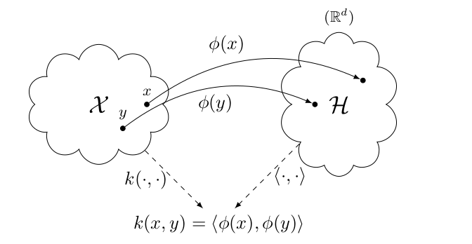
Reproducing kernel Hilbert space (RKHS). Let \(\mathcal{X}\) be a non empty set and \(k\) be a positive definite kernel on \(\mathcal{X}\). A Hilbert space \(\mathcal{H}_k\) of function on \(\mathcal{X}\) equipped with an inner product \(\langle ., . \rangle_{\mathcal{H}_k}\) is called a reproducing kernel Hilbert space (RKHS) with reproducing kernel \(k\), if the following are satisfied:

1. For all \(x \in \mathcal{X}\), we have \(k(., x) \in \mathcal{H}_k\).
2. For all \(x \in \mathcal{X}\), and for all \(f \in \mathcal{H}_k\)

Martingale. Martingale is a stochastic process \(X_1, \dots, X_N\) that satisfies for any time \(n\),

that is, the condition expected value of the next observation, given all the history is determined only by the current observation.

This agnostic setting introduces key differences compared to the previous one:

1. Function space: \(f\) is no longer restricted to sample drawn from a GP. Instead, it can be an arbitrary function from \(\mathcal{H}_k(D)\).
2. Noise model relaxation: While UCB assumes that the noise \(\epsilon_t = y_t - f(x_t)\) is drawn independently from \(N(0, \sigma^2)\), we relax the assumption such that the sequence of noise variables can be a uniformly bounded martingale difference sequence: \(\epsilon_t \leq \sigma\) for all \(t \in \mathbb{N}\).

Regret Bound for the Function in RKHS

Theorem 3 Let \(\delta \in (0, 1)\). Assume that the true underflying \(f\) lies in RKHS \(\mathcal{H}_k(D)\) corresponding to the kernel \(k(x, x^\prime)\) and the noise \(\epsilon_t\) has zero mean conditioned on the history and is bounded by \(\sigma\) almost surely. In particular, assume \(\Vert f \Vert_k^2 \leq B\) and let \(\beta_t = 2B + 300 \gamma_t \log^3 (t / \delta)\). Running GP-UCB with \(\beta_t\), prior \(GP(0, k(x, x^\prime))\) and noise model \(N(0, \sigma^2)\), we obtain a regret bound of \(\mathcal{O}(\sqrt{T}(B \sqrt{\gamma_T} + \gamma_T))\) with high probability. Precisely,

where \(C_1 = 8 / \log(1 + \sigma^{-2})\).

Proof:

Given the posterior covariance \(k_T(., .)\), we have

It implies that \(\mathcal{H}_k(D) = \mathcal{H}_{k_T}(D)\), while \(\Vert f \Vert_{k_T} \leq \Vert f \Vert_{k}\). By the reproducing property and Cauchy-Schwarz inequality, we have

We need to lift up Theorem 1 to the agnostic setting in order to prove Theorem 3. For that purpose, it requires the following theorem to have an equivalence of Lemma 5.1 (see Part I).

Theorem 6 Let \(\delta \in (0, 1)\). Assume the noise variance \(\epsilon_t\) are uniformly bounded by \(\sigma\). Define

Then

Proof:

The strategy is to show that

Theorem 6 will follow from \eqref{eq:rkhs-inequality}. The proof analyzes the quantity \(Z_T\) and then bounds the martiangle difference.

Bound of \(Z_t\)

We first analyze the quantity \(Z_T = \Vert \mu_T - f \Vert_{k_T}^2\), that is the error of \(\mu_T\) as the approximation of \(f\) under the RKHS norm \(\mathcal{H}_{k_T}(D)\). The analysis requires a lemma which is responsible to bound the growth of \(Z_T\). Establishing this lemma requires normalized quantities: \(\tilde{\epsilon}_t = \epsilon_t / \sigma, \tilde{f} = f / \sigma, \tilde{\mu}_t = \mu_t / \sigma, \tilde{\sigma}_t = \sigma_t / \sigma\). For convenience, \(\mu_{t - 1}\) and \(\sigma_{t - 1}\) are the shorthand for \(\mu_{t - 1}(x_t)\) and \(\sigma_{t - 1}(x_t)\), respectively.

Lemma 7.2 For all \(T \in \mathbb{N}\),

Proof:

If \(\boldsymbol{\alpha}_t = (\mathbf{K}_t + \sigma^2 \mathbf{I})^{-1} \mathbf{y}_t\), then \(\mu_t(x) = \boldsymbol{\alpha}_t^\top \mathbf{k}_t(x)\). Moreover, we have \(\langle \mu_T, f \rangle_k = \mathbf{f}^\top_T \boldsymbol{\alpha}_T, \Vert \mu_T \Vert^2_k = \mathbf{y}_T^\top \boldsymbol{\alpha}_T - \sigma^2 \Vert \boldsymbol{\alpha}_T \Vert^2, \mu_T(x_t) = \boldsymbol{\delta}_t^\top \mathbf{K}_T (\mathbf{K}_T + \sigma^2 \mathbf{I})^{-1} \mathbf{y}_T = y_t - \sigma^2 \alpha_t\). Since \(Z_T = \Vert \mu_T - f \Vert_k + \sigma^{-2} \sum_{t \leq T} (\mu_T(x_t) - f(x_t))^2\), we have

Note that \(2 \log p(\mathbf{y}_t) \propto - \mathbf{y}_T^\top (\mathbf{K}_T + \sigma^2 \mathbf{I})^{-1} \mathbf{y}_T\). Since \(\log p(\mathbf{y}_T) = \sum_{t = 1} \log p(y_t \vert \mathbf{y}_{< t}) = \sum_t \log N(y_t \vert \mu_{t - 1}(x_t), \sigma^2_{t - 1}(x_t) + \sigma^2)\), we have

with \(R = \sum_t (\mu_{t - 1} - f(x_t))^2 / (\sigma^2 + \sigma^2_{t - 1}) \geq 0\). Dropping \(-R\) and changing to normalized quantities concludes the proof.

Concentration of Martingale

We need the following lemma to construct the proof of Lemma 7.3.

Lemma 7.1 We have that

Proof:

We have that \(\min(r, \alpha) \leq (\alpha / \log(1 + \alpha)) \log (1 + r)\). The statement follows from Lemma 5.3. (see Part I)

We also need the concentration inequality for martingale differences:

Theorem 7 (Freedman) Suppose \(X_1, \dots, X_T\) is a martingale difference sequence, and \(b\) is an uniform upper bound on the steps \(X_i\). Let \(V\) denote the sum of conditional variances,

Then, for every \(a, v > 0\),

We now define a martingale difference sequence. First, we define the “escape-event” \(E_T\) as

Subsequently, we define the random variables \(M_t\) by

Remark: Since \(\tilde{\epsilon}_t\) is a martingale difference sequence w.r.t. the histories and \(M_t / \tilde{\epsilon}_t\) is deterministic given the history, \(M_t\) is martingale difference sequence as well.

The following lemma tells with a high probability, the associated martingale \(\sum_{t = 1}^T M_t\) does not grow too large.

Lemma 7.3 Given \(\delta \in (0, 1)\) and \(\beta_t\) as defined in Theorem 6, we have that

Proof:

We first obtain upper bound on the step sizes of the martingale.

The first inequality follows from \eqref{eq:rkhs-inequality} and the definition of \(E_t\). The second inequality follows from the fact that \(r / (1 + r^2) \leq \min\{r, 1/2 \}\) for \(r \geq 0\). Thus, \(\vert M_t\vert \leq \beta_{T}^{1 / 2}\) since \(\vert \tilde{\epsilon} \vert \leq 1\) and \(\beta_t\) is non-decreasing. Next, we bound the sum of the conditional variances of the martingale:

The last inequality follows from Lemma 7.1, with \(\alpha=1/4\). We then apply Theorem 7 with parameters \(a = \beta_{T + 1} / 2, b = \beta_{T + 1}^{1 / 2}\), and \(v = 9 \beta_T \gamma_T\) to obtain

Note that \(\beta_{T + 1}\) satisfies

Therefore, the previous probability is bounded by \(\delta / T^2\). By applying the union bound we obtain

completing the proof of Lemma 7.3.

[Proof of Theorem 6] By Lemma 7.2 and the definition of \(\beta_1\), we have \(Z_0 \leq \Vert f \Vert_k \leq \beta_1\). Hence, we always have \(E_0 = 1\). Suppose with a high-probability Lemma 7.3 holds, i.e., \(\sum_t M_t \leq \beta_{T + 1} / 2\). For the inductive hypothesis, assume \(E_T = 1\). By applying Lemma 7.2 we obtain

The equality in the second step uses the inductive hypothesis. Thus we have shown \(E_T = 1\), completing the induction.

Following the proof of Theorem 1 and replacing Lemma 5.1 with Theorem 6 leads to the results in Theorem 3. Note that Theorem 3 holds uniformly over all functions \(f\), with \(\Vert f \Vert < \infty\).

In the last part of this blog series, we aim to obtain the bound the quantity \(\gamma_T\) for practical classes of kernels.

Reference

• Srinivas, N., Krause, A., Kakade, S. M., & Seeger, M. (2009). Gaussian process optimization in the bandit setting: No regret and experimental design. arXiv preprint arXiv:0912.3995.